This post was inspired by and draws heavily from the material in the Python Graph Gallery, specifically the page on 2D density plots. I highly recommend checking out that page as well as the other pages on the Python Graph Gallery.

Visualizing the relationship between two variables based on a collection of observations is one of the most common tasks performed by data scientists. In many cases, the humble scatter plot works well for this purpose. However, when the number of data points being visualized is large, scatter plots with overlapping points become saturated and the relationship between the two variables can be lost in a blob of overlapping points.

To get us started seeing how 2D density plots work, let’s import a few libraries that we are going to need and center plots on the page so that they look nice.

# import libraries and set matplotlib inline magic
import numpy as np
import matplotlib.pyplot as plt
from scipy.stats import kde
%matplotlib inline

First, let’s just look at some randomly generated data.

# Draw 10000 points from a multivariate normal distribution
num_points = 100
mean_x = 0
mean_y = 0
cov_xx = 1
cov_xy = 0.5
cov_yy = 3

#                multivariate_normal(mean_vector, covariance_matrix, size)
data = np.random.multivariate_normal([mean_x, mean_y], [[cov_xx, cov_xy], [cov_xy, cov_yy]], num_points)
x, y = data.T

An ordinary scatter plot of this data might look something like this:

plt.figure(figsize=(8,8))
plt.scatter(x,y)

<matplotlib.collections.PathCollection at 0x1a1f678518>

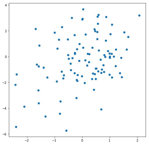
With these settings and just 100 data points, visualizing this data with a scatter plot works pretty well. Although the relationship between the two variables may not be clearly discernible, this is probably not the fault of the visualization, per se. Rather, we may just have too few observations to say anything definite about the relationship. So let’s collect some more data and plot it again.

num_points = 1000
data = np.random.multivariate_normal([mean_x, mean_y], [[cov_xx, cov_xy], [cov_xy, cov_yy]], num_points)
x, y = data.T
plt.figure(figsize=(8,8))
plt.scatter(x,y)

<matplotlib.collections.PathCollection at 0x1a203602e8>

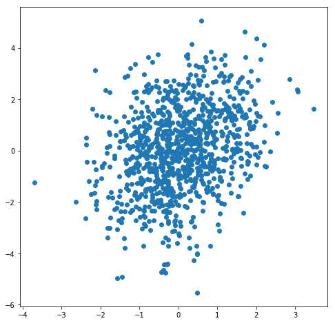
With 1000 data points, we are starting to see the relationship more clearly. And the plot is not yet too crowded, although the points are now certainly starting to overlap. If we wanted to gain more confidence in our understanding of the relationship between these two variables, we might choose to collect even more data, so let’s give it a try.

num_points = 10000
data = np.random.multivariate_normal([mean_x, mean_y], [[cov_xx, cov_xy], [cov_xy, cov_yy]], num_points)
x, y = data.T
plt.figure(figsize=(8,8))
plt.scatter(x,y)

<matplotlib.collections.PathCollection at 0x1a203c5048>

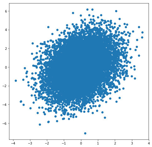
At this point, the plot is very crowded and there is a lot of information being lost in the middle of the plot where it is completely saturated. What if we try shrinking the size of the points?

plt.figure(figsize=(8,8))
plt.scatter(x,y,s=5)

<matplotlib.collections.PathCollection at 0x1a203f80f0>

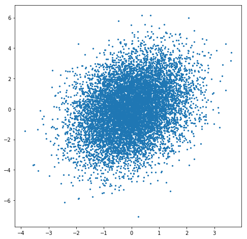
That definitely helps. Now we can see that the points are more dense in the middle than around the edges and, perhaps if you squint, that the points are more dense in the first and third quadrants than they are in the second and fourth quadrants. But can we do better? Perhaps the simplest solution is to create a 2D histogram of the points. Let’s give that a try.

# 2D Histogram
nbins=10

plt.figure(figsize=(10,8))
plt.title('2D Histogram')
fig = plt.hist2d(x, y, bins=nbins, cmap='Blues')
plt.colorbar()

<matplotlib.colorbar.Colorbar at 0x1a20c962b0>

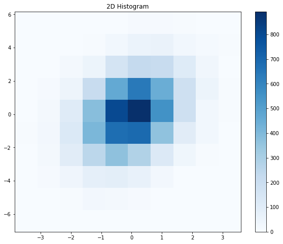
Probably the first thing that you’ll notice is that the data looks quite “blocky”. This is a good way of illustrating one of the caveats that will come along with converting scatter plots to density plots: there will always be, whether it is hidden from you or not, some assumptions about the data that go into producing a density plot from a set of points. In the case of the 2D histogram, these assumptions are in plain sight, which I consider a strength of the 2D histogram. At the top of the previous code cell, we specified the nbins variable. Let’s see how changing the nbins variable affects the look of the plot.

nbins=100

plt.figure(figsize=(10,8))
plt.title('2D Histogram')
fig = plt.hist2d(x, y, bins=nbins, cmap='Blues')
plt.colorbar()

<matplotlib.colorbar.Colorbar at 0x1a213714a8>

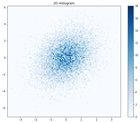
As you can see, if we set the nbins variable too high, then the histogram doesn’t look much better than the original scatter plot. What about nbins=20?

nbins=20

plt.figure(figsize=(10,8))
plt.title('2D Histogram')
fig = plt.hist2d(x, y, bins=nbins, cmap='Blues')
plt.colorbar()

<matplotlib.colorbar.Colorbar at 0x1a2291bda0>

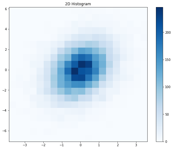
This seems like a pretty good value for this data set. I would argue that the relationship between the two variables is more evident based on the 2D histogram than it was from the raw scatter plot. It is clear that the points are concentrated around x=0, y=0 and that the points are spread around x=y. Can we do even better? If you recall (or you look above), using nbins=100 with a straightforward 2D histogram resulted in a plot that looked very noisy. This is understandable, as we are building our plot based on finite sampling of two random variables. Can we “smooth out” the data in a reasonable way without performing more sampling? Kernel density estimation, or KDE, is one means of smoothing data. Let’s see how applying KDE affects the look of our plot.

# Evaluate a gaussian kde on a regular grid of nbins x nbins over data extents
nbins = 100

k = kde.gaussian_kde(data.T)
xi, yi = np.mgrid[x.min():x.max():nbins*1j, y.min():y.max():nbins*1j]
zi = k(np.vstack([xi.flatten(), yi.flatten()]))

# 2D density plot without added shading
plt.figure(figsize=(8,8))
plt.title('2D Density with kernel density estimation')
plt.pcolormesh(xi, yi, zi.reshape(xi.shape), cmap='Blues')

<matplotlib.collections.QuadMesh at 0x1a238e27f0>

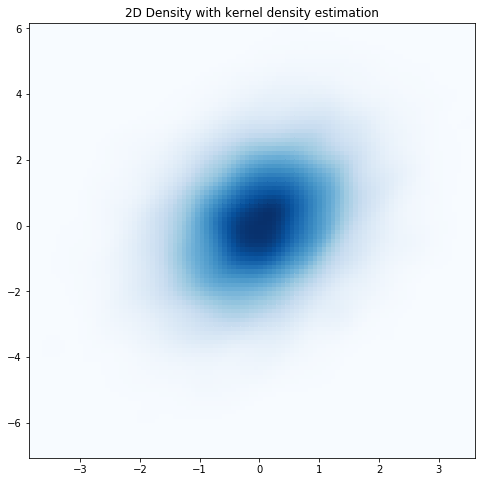
With KDE applied, even with nbins=100 the data looks smooth. So, free lunch? Not exactly. As I mentioned above, there are always assumptions that go into converting scatter plots to density plots. Quoting from the SciPy website:

(KDE) includes automatic bandwidth determination. The estimation works best for a unimodal distribution; bimodal or multi-modal distributions tend to be oversmoothed.

The “automatic bandwidth determination” mentioned there is the equivalent of the fiddling around that we did with the nbins with the 2D histogram. Real data might not be unimodal, so it is probably best to look at some of the more “raw” visualizations (scatter plots and ordinary histograms) even if you eventually go with using KDE for your final visualization.

If you look closely, you can still see the granularity resulting from the binning even with a large number of bins and with KDE applied. Matplotlib allows you to interpolate the colors within bins using something called “Gouraud shading”. Let’s give it a try.

# Evaluate a gaussian kde on a regular grid of nbins x nbins over data extents
nbins = 100

# 2D density plot with added shading
plt.figure(figsize=(8,8))
plt.title('2D Density with Gouraud shading')
plt.pcolormesh(xi, yi, zi.reshape(xi.shape), shading='gouraud', cmap='Blues')

<matplotlib.collections.QuadMesh at 0x1a23bbdba8>

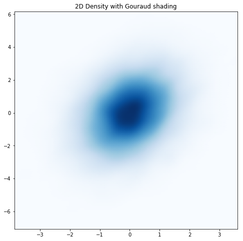
Very smooth! Is there anything else that we might want to add? In my opinion, although our latest plot looks nice, for some people it may not do as good of a job conveying the relationship between the two variables. Let’s add some contour lines to see how that might help (while allowing us to keep the smoothed representation of our data).

# Evaluate a gaussian kde on a regular grid of nbins x nbins over data extents
nbins = 100

# 2D density plot with added shading
plt.figure(figsize=(8,8))
plt.title('2D Density with contour lines')
plt.pcolormesh(xi, yi, zi.reshape(xi.shape), shading='gouraud', cmap='Blues')
plt.contour(xi, yi, zi.reshape(xi.shape))

<matplotlib.contour.QuadContourSet at 0x1a23ed2828>

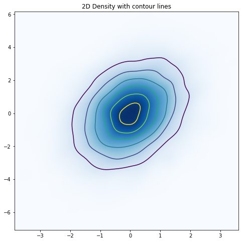
With the contour lines in place, it is very clear that we are dealing with a multivariate normal distribution with positive covariance along x=y. So should you always just skip immediately to this representation of the data? I don’t think so. As data scientists, we are responsible for making sure that the representation of the data that we are showing is faithful to the underlying data. Because we apply assumptions to derive density plots from raw data, it is a good idea to gradually abstract the data (as we did in this post) to ensure that the final visualization is a good representation of the data. Finally, these density plots are only useful if the density of the data is what you are mostly interested in. Other types of scatter plots, where, for example, you make use of the color and/or size of the points, may be more useful depending upon what you are interested in visualizing.

As I mentioned at the top of the post, this post was inspired by the 2D density plots page at the Python Graph Gallery. Go have a look!